Category Archives: Physics

Interpreting the Quantum World I: Measurement & Non-Locality

In previous posts Aron introduced us to the strange, yet compelling world of quantum mechanics and its radical departures from our everyday experience. We saw that the classical world we grew up with, where matter is composed of solid particles governed by strictly deterministic equations of state and motion, is in fact somewhat “fuzzy.” The atoms, molecules, and subatomic particles in the brightly colored illustrations and stick models of our childhood chemistry sets and schoolbooks are actually probabilistic fields that somehow acquire the properties we find in them when they’re observed. Even a particle’s location is not well-defined until we see it here, and not there. Furthermore, because they are ultimately fields, they behave in ways the little hard “marbles” of classical systems cannot, leading to all sort of paradoxes. Physicists, philosophers, and theologians alike have spent nearly a century trying to understand these paradoxes. In this series of posts, we’re going to explore what they tell us about the universe, and our place in it.

To quickly recap earlier posts, in quantum mechanics (QM) the fundamental building block of matter is a complex-valued wave function \(\Psi\) whose squared amplitude is a real-valued number that gives the probability density of observing a particle/s in any given state. \(\Psi\) is most commonly given as a function of the locations of its constituent particles, \(\Psi\left ( \vec{r_{1}}, \vec{r_{2}}… \vec{r_{n}} \right )\), or their momentums, \(\Psi\left ( \vec{p_{1}}, \vec{p_{2}}… \vec{p_{n}} \right )\) (but not both, which as we will see, is important), but will also include any of the system’s other variables we wish to characterize (e.g. spin states). The range of possible configurations these variables span is known as the system’s Hilbert space. As the system evolves, its wave function wanders through this space exploring its myriad probabilistic possibilities. The time evolution of its journey is derived from its total energy in a manner directly analogous to the Hamiltonian formalism of classical mechanics, resulting in the well-known time-dependent Schrödinger equation. Because \(\left | \Psi \right |^{2}\) is a probability density, its integral over all of the system’s degrees of freedom must equal 1. This irreducibly probabilistic aspect of the wave function is known as the Born Rule (after Max Born who first proposed it), and the mathematical framework that preserves it in QM is known as unitarity. [Fun fact: Pop-singer Olivia Newton John is Born’s granddaughter!]

Notice that \(\Psi\) is a single complex-valued wave function of the collective states of all its constituent particles. This makes for some radical departures from classical physics. Unlike a system of little hard marbles, it can interfere with itself—not unlike the way the countless harmonics in sound waves give us melodies, harmonies, and the rich tonalities of Miles Davis’ muted trumpet or Jimi Hendrix’s Stratocaster. The history of the universe is a grand symphony—the music of the spheres! Its harmonies also lead to entangled states, in which one part may not be uniquely distinguishable from another. So, it will not generally be true that the wave function of the particle sum is the sum of the individual particle wave functions,

\(\Psi\left ( \vec{r_{1}}, \vec{r_{2}}… \vec{r_{n}} \right ) \neq \Psi\left ( \vec{r_{1}} \right )\Psi\left ( \vec{r_{2}} \right )… \Psi\left ( \vec{r_{n}} \right )\)

until the symphony progresses to a point where individual particle histories decohere enough to be distinguished from each other—melodies instead of harmonies.

Another consequence of this wave-like behavior is that position and momentum can be converted into each other with a mathematical operation known as a Fourier transform. As a result, the Hilbert space may be specified in terms of position or momentum, but not both, which leads to the famous Heisenberg Uncertainty principle,

\(\Delta x\Delta p \geqslant \hbar/2\)

where \(\hbar\) is the reduced Planck constant. It’s important to note that this uncertainty is not epistemic—it’s an unavoidable consequence of wave-like behavior. When I was first taught the Uncertainty Principle in my undergraduate Chemistry series, it was derived by modeling particles as tiny pool ball “wave packets” whose locations couldn’t be observed by bouncing a tiny cue-ball photon off them without batting them into left field with a momentum we couldn’t simultaneously see. As it happens, this approach does work, and is perhaps easier for novice physics and chemistry students to wrap their heads around. But unfortunately, it paints a completely wrong-heading picture of the underlying reality. We can pin down the exact location of a particle, but in so doing we aren’t simply batting it away—we’re destroying whatever information about momentum it originally had, rendering it completely ambiguous, and vice versa (in the quantum realm paired variables that are related to each other like this are said to be canonical). The symphony is, to some extent, irreducibly fuzzy!

So… the unfolding story of the universe is a grand symphony of probability amplitudes exploring their Hilbert space worlds along deterministic paths, often in entangled states where some of their parts aren’t entirely distinct from each other, and acquiring whatever properties we find them to have only when they’re measured, many of which cannot simultaneously have exact values even in principle. Strange stuff to say the least! But the story doesn’t end there. Before we can decipher what it all means (or, I should say, get as close as doing so as we ever will) there are two more subtleties to this bizarre quantum world we still need to unpack… measurement and non-locality.

Measurement

The first thing we need to wrap our heads around is observation, or in quantum parlance, measurement. In classical systems matter inherently possesses the properties that it does, and we discover what those properties are when we observe them. My sparkling water objectively exists in a red glass located about one foot to the right of my keyboard, and I learned this by looking at it (and roughly measuring the distance with my thumb and fingers). In the quantum realm things are messier. My glass of water is really a bundle of probabilistic particle states that in some sense acquired its redness, location, and other properties by the very act of my looking at it and touching it. That’s not to say that it doesn’t exist when I’m not doing that, only that its existence and nature aren’t entirely independent of me.

How does this work? In quantum formalism, the act of observing a system is described by mathematical objects known as operators. You can think of an operator as a tool that changes one function into another one in a specific way—like say, “take the derivative and multiply by ten.” The act of measuring some property \(A\) (like, say, the weight or color of my water glass) will apply an associated operator \(\hat A\) to its initial wave function state \(\Psi_{i}\) and change it to some final state \(\Psi_{f}\),

\(\hat A \Psi_{i} = \Psi_{f}\)

For every such operator, there will be one or more states \(\Psi_{i}\) could be in at the time of this measurement for which \(\hat A\) would end up changing its magnitude but not its direction,

\(\begin{bmatrix} \hat A \Psi_{1} = a_{1}\Psi_{1}\\ \hat A \Psi_{2} = a_{2}\Psi_{2}\\ …\\ \hat A \Psi_{n} = a_{n}\Psi_{n} \end{bmatrix}\)

These states are called eigenvectors, and the constants \(a_{n}\) associated with them are the values of \(A\) we would measure if \(\Psi\) is in any of these states when we observe it. Together, they define a coordinate system associated with \(A\) in the Hilbert space that \(\Psi\) can be specified in at any given moment in its history. If \(\Psi_{i}\) is not in one of these states when we measure \(A\), doing so will force it into one of them. That is,

\(\hat A \Psi_{i} \rightarrow \Psi_{n}\)

and \(a_{n}\) will be the value we end up with. The projection of \(\Psi_{i}\) on any of the \(n\) axes gives the probability amplitude that measuring \(A\) will put the system into that state with the associated eigenvalue being what we measure,

\(P(a_{n}) = \left | \Psi_{i} \cdot \Psi_{n} \right |^{2}\)

So… per the Schrödinger equation, our wave function skips along its merry, deterministic way through a Hilbert space of unitary probabilistic states. Following a convention used by Penrose (2016), let’s designate this part of the universe’s evolution as \(\hat U\). All progresses nicely, until we decide to measure something—location, momentum, spin state, etc. When we do, our wave function abruptly (some would even be tempted to say magically) jumps to a different track and spits out whatever value we observe, after which \(\hat U\) starts over again in the new track.

This event—let’s call it \(\hat M\)—has nothing whatsoever to do with the wave function itself. The tracks it jumps to are determined by whatever properties we observe, and the outcome of these jumps are irreducibly indeterminate. We cannot say ahead of time which track we’ll end up on even in principle. The best we can do is state that some property \(A\) has such and such probability of knocking \(\Psi\) into this or that state and returning its associated value. When this happens, the wave function is said to have “collapsed.” [Collapsed is in quotes here for a reason… as we shall see, not all interpretations of quantum mechanics accept that this is what actually happens!]

Non-Locality

It’s often said that quantum mechanics only applies to the subatomic world, but on the macroscopic scale of our experience classical behavior reigns. For the most part this is true. But… as we’ve seen, \(\Psi\) is a wave function, and waves are spread out in space. Subatomic particles are only tiny when we observe them to be located somewhere. So, if \(\hat M\) involves a discrete collapse, it happens everywhere at once, even over distances that according to special relativity cannot communicate with each other—what some have referred to as “spooky action at a distance.” This isn’t mere speculation, nor a problem with our methods—it can be observed.

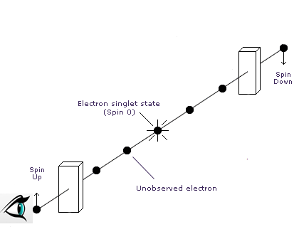
Consider two electrons in a paired state with zero total spin. Such states (which are known as singlets) may be bound or unbound, but once formed they will conserve whatever spin state they originated with. In this case, since the electron cannot have zero spin, the paired electrons would have to preserve antiparallel spins that cancel each other. If one were observed to have a spin of, say, +1/2 about a given axis, the other would necessarily have a spin of -1/2. Suppose we prepared such a state unbound, and sent the two electrons off in opposite direction. As we’ve seen, until the spin state of one of them is observed, neither will individually be in any particular spin state. The wave function will be an entangled state of two possible outcomes, +/- and -/+ about any axis. Once we observe one of them and find it in, say, a “spin-up” state (+1/2 about a vertical axis), the wave function will have collapsed to a state in which the other must be “spin-down” (-1/2), and that will be what we find if it’s observed a split second later as shown below.

But what would happen if the two measurements were made over a distance too large for a light signal to travel from the first observation point to the second one during the time delay between the two measurements? Special relativity tells us that no signal can communicate faster than the speed of light, so how would the second photon know that it was supposed to be in a spin-down state? Light travels 11.8 inches in one nanosecond, so it’s well within existing microcircuit technology to test this, and it has been done on many occasions. The result…? The second photon is always found in a spin state opposite that of the first. Somehow, our second electron knows what happened to its partner… instantaneously!

If so, this raises some issues. Traditional QM asserts that the wave function gives us a complete description of a system’s physical reality, and the properties we observe it to have are instantiated when we see them. At this point we might ask ourselves two questions;

1)  How do we really know that prior to our observing it, the wave function truly is in an entangled state of two as-yet unrealized outcomes? What if it’s just probabilistic scaffolding we use to cover our lack of understanding of some deeper determinism not captured by our current QM formalism?

2)  What if the unobserved electron shown above actually had a spin-up property that we simply hadn’t learned about yet, and would’ve had it whether it was ever observed or not (a stance known as counterfactual definiteness)? How do we know that one or more “hidden” variables of some sort hadn’t been involved in our singlet’s creation, and sent the two electrons off with spin state box lunches ready for us to open without violating special relativity (a stance known as local realism)?

Together, these comprise what’s known as local realism, or what Physicist John Bell referred to as the “Bertlmann’s socks” view (after Reinhold Bertlmann, a colleague of his at CERN). Bertlmann was known for never wearing matching pairs of socks to work, so it was all but guaranteed that if one could observe one of his socks, the other would be found to be differently colored. But unlike our collapsed electron singlet state, this was because Bertlmann had set that state up ahead of time when he got dressed… a “hidden variable” one wouldn’t be privy to unless they shared a flat with him. His socks would already have been mismatched when we discovered them to be, so no “spooky action at a distance” would be needed to create that difference when we first saw them.

In 1964 Bell proposed a way to test this against the entangled states of QM. Spin state can only be observed in one axis at a time. Our experiment can look for +/- states about any axis, but not together. If an observer “Alice” finds one of the electrons in a spin-up state, the second photon will be in a spin-down state. What would happen if another observer “Bob” then measured its spin state about an axis at, say, a 45-deg. angle to vertical as shown below?

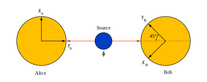
The projection of the spin-down wave function on the eigenvector coordinate system of Bob’s measurement will translate into probabilities of observing + or – states in that plane. Bell produced a set of inequalities bearing his name which showed that if the electrons in our singlet state had in fact been dressed in different colored socks from the start, experiments like this will yield outcomes that differ statistically from those predicted by traditional QM. This too has been tested many times, and the results have consistently favored the predictions of QM, leaving us with three options;

a)  Local realism is not valid in QM. Particles do not inherently possess properties prior to our observing them, and indeterminacy and/or some degree of “spooky action at a distance” cannot be fully exorcised from \(\hat M\).

b)  Our understanding of QM is incomplete. Particles do possess properties (e.g. spin, location, or momentum) whether we observe them or not (i.e. – counterfactuals about measurement outcomes exist), but our understanding of \(\hat U\) and \(\hat M\) doesn’t fully reflect the local realism that determines them.

c)  QM is complete, and the universe is both deterministic and locally real without the need for hidden variables, but counterfactual definiteness is an ill-formed concept (as in the “Many Worlds Interpretation” for instance).

Nature seems to be telling us that we can’t have our classical cake and eat it. There’s only room on the bus for one of these alternatives. Several possible loopholes have been suggested to exist in Bell’s inequalities through which underlying locally real mechanics might slip through. These have led to ever more sophisticated experiments to close them, which continue to this day. So far, the traditional QM frameworks has survived every attempt to up the ante, painting Bertlmann’s socks into an ever-shrinking corner. In 1966, Bell, and independently in 1967, Simon Kochen and Ernst Specker, proved what has since come to be known as the Kochen-Specker Theorem, which tightens the noose around hidden variables even further. What they showed, was that regardless of non-locality, hidden variables cannot account for indeterminacy in QM unless they’re contextual. Essentially, this all but dooms counterfactual definiteness in \(\hat M\). There are ways around this (as there always are if one is willing to go far enough to make a point about something). The possibility of “modal” interpretations of QM have been floated, as has the notion of a “subquantum” realm where all of this is worked out. But these are becoming increasingly convoluted, and poised for Occam’s ever-present razor. As of this writing, hidden variables theories aren’t quite dead yet, but they are in a medically induced coma.

In case things aren’t weird enough for you yet, note that a wave function collapse over spacelike distances raises the specter of the relativity of simultaneity. Per special relativity, over such distances the Lorentz boost blurs the distinction between past and future. In situations like these it’s unclear whether the wave function was collapsed by the first observation or the second one, because which one is in the future of the other is a matter of which inertial reference frame one is viewing the experiment from. Considering that you and I are many-body wave functions, anything that affects us now, like say, stubbing a toe, collapses our wave function everywhere at once. As such, strange as it may sound, in a very real sense it can be said that a short while ago your head experienced a change because you stubbed your toe now, not back then. And… It will experience a change shortly because you did as well. Which of these statements is correct depends only on the frame of reference from which the toe-stubbing event is viewed. It’s important to note that this has nothing to do with the propagation of information along our nerves—it’s a consequence of the fact that as “living wave functions”, our bodies are non-locally spread out across space-time to an extent that slightly blurs the meaning of “now”.  Of course, the elapsed times associated with the size of our bodies are too small to be detected, but the basic principle remains.

Putting it all together

Whew… that was a lot of unpacking! And the world makes even less sense now than it did when we started. Einstein once said that he wanted to know God’s thoughts, the rest were just details. Well it seems the mind of God is more inscrutable than we ever imagined! But now we have the tools we need to begin exploring some of the way His thoughts have been written into the fabric of creation. Our mission, should we choose to accept it, is to address the following;

1)  What is this thing we call a wave function? Is it ontologically real, or just mathematical scaffolding we use to make sense of things we don’t yet understand?

2)  What really happens when a deterministic, well-behaved \(\hat U\) symphony runs headlong into a seemingly abrupt, non-deterministic \(\hat M\) event? How do we get them to share their toys and play nicely with each other?

3)  If counterfactual definiteness is an ill-formed concept and every part of the wave function is equally real, why do our observations always leave us with only one experienced outcome? Why don’t we experience entangled realities, or even multiple realities?

In the next installment in this series we’ll delve into a few of the answers that have been proposed so far. The best is yet to come, so stay tuned!

References

Penrose, R. (2016). Fashion, faith, and fantasy in the new physics of the universe. Princeton University Press, Sept. 13, 2016. ISBN: 0691178534; ASIN: B01AMPQTRU. Available online at www.amazon.com/Fashion-Faith-Fantasy-Physics-Universe-ebook/dp/B01AMPQTRU/ref=sr_1_1?ie=UTF8&qid=1495054176&sr=8-1&keywords=penrose. Accessed June 11, 2017.

Open and Closed

A reader asks:

This seems to be as good a place as any to ask a question about closed universes.

See, in a lot of popular science books, they teach you that an “open” universe is one where space is infinite, saddle-shaped, and keeps expanding forever; a “flat” universe is infinite, plane-shaped, and the rate of expansion eventually peters out to zero; and a “closed” universe is finite, sphere-shaped, and eventually contracts in a big crunch. They then talk about the cosmological constant and “dark energy,” which make our universe expand at an accelerating rate, something that doesn’t fit the taxonomy of possibilities for the universe’s topology, and which they do not relate back to that taxonomy in any way.

Can a universe with lots of dark energy be a closed universe? Will a closed universe with dark energy keep on expanding and accelerating, or will it eventually collapse in a big crunch like a “normal” closed universe? Is the three-type Taxonomy only relevant given certain energy conditions? (Strong/weak/null)

Oh, and I almost forgot:

are there any good reasons to think that the universe is closed in the first place, other than Kalam-esqe arguments against actual infinities?

David,
It sounds like these books were just adding the new material about the cosmological constant to the old discussions without doing the hard work of going back and revising it so that it makes sense.

The Bad Old Days

In the old days (pre circa 1998) people didn’t know about the acceleration of the universe, and they thought that the universe just consisted of ordinary radiation and matter (where for these purposes, dark matter is a form of matter).  In the old days, the model of closed, flat, and open works exactly as you say: a closed universe (spherical geometry) will recollapse, and open one (hyperbolic geometry) will trend to a constant rate of expansion (in terms of distance / time) and a flat one is right on the edge and will expand forever at a slower and slower rate (but still getting arbitrarily large).

Given the rate of expansion, it takes a certain amount of energy density to get a flat universe.  Too much, and you get a sphere, too little and you get hyperbolic space.  (The expansion or contraction of the universe makes it hyperbolic in the absence of matter.)  These are the 3 kinds of geometries which are homogeneous (the same everywhere) and isotropic (the same in every direction).  On average, the observable universe seems to be homogenous and isotropic, so it’s got to be one of these three (a.k.a. an “FRW cosmology”).

However, this was confusing for several reasons.  One is that the cosmological data kept suggesting that there wasn’t enough energy in matter to get anywhere close to a flat universe, yet other data seemed more consistent with a flat universe.  A flat universe is also a natural consequence of inflation since it stretches out the pre-existing geometry to exponentially large distance scales.  Also, the universe seemed like it wasn’t quite old enough to explain all the structures in it.

Concordance Cosmology

Now we know that there is an additional form of energy which is confusingly called “dark energy” (but I dislike this name, because it makes people think it has something to do with “dark matter”.)  Most likely it is just a cosmological constant, a constant energy density in all of space.

Now it turns out that for purposes of determining the spatial geometry, a positive cosmological constant counts positively (so it helps to close the universe).  But when you calculate its effect on the expansion of the universe, it counts negatively, as repulsive gravity.

This may seem like odd behavior because energy and mass are equivalent, and we all know that mass causes gravitational attraction, not repulsion.  But in turns out that in General Relativity, both energy density (associated with time) and pressure (associated with space) lead to attractive gravity.  Negative pressure is called tension, and tension therefore causes antigravity.

In ordinary matter travelling at low speeds, the amount of pressure/tension is typically very small compared to the energy density.  Radiation which travels near the speed of light has a lot of pressure, but that only makes gravity stronger.

On the other hand, a positive cosmological constant has tension equal to its energy density.  Something has tension if, when you stretch it out, it’s energy increases.  But the energy of the cosmological constant is proportional to the volume, so when the volume increases the energy increases proportionally.  Hence the tension in each spatial direction is equal to the energy.  Since there are 3 dimensions of space and only 1 of time, the antigravity due to the tension is 3 times larger than the gravity due to the energy density.  Hence the antigravity wins!  So paradoxically, the gravitational effects of this tension just make the universe want to grow faster!  Unlike the usual effects of tension, which cause things to shrink in on themselves.

On the other hand, if the cosmological constant were negative (it isn’t, but suppose) its effects would be reversed: it would make the spatial geometry more hyperbolic, but would decelerate the expansion.

So, once you include a cosmological constant, the rules change (as you guessed).  You can still have the same 3 types of spatial geometry (the words “open”, “flat”, and “closed” describe the spatial geometry, not the dynamics).  But with a positive cosmological constant, even a universe with closed topology can sometimes expand forever, if it gets big enough for the cosmological constant to take over.  (Matter thins out, while the CC doesn’t, so when the universe is small the matter is more important, and when it gets larger the CC is more important.)  On the other hand, with a negative cosmological constant, even an open cosmology will always eventually recollapse when it gets big enough.

(The various energy conditions you mention place limits on the allowed energy density and/or tension/pressure, so not surprisingly these have certain implications for what a cosmology can do.  Note that a positive CC violates the strong energy condition—which allows for a bounce, at least in the case of a closed universe.  While a negative CC violates the weak energy condition, which requires that any FRW cosmology which is neither expanding nor contracting at some time, must be closed.  (OK, technically it also allows space to be flat, but only if the matter energy is exactly 0, which is unrealistic.))

Our universe seems to have a positive cosmological constant, which fixes all of the problems I mentioned above.  The cosmological constant seems to give us exactly the extra energy density we need to get a flat universe.  Yet it also causes the universe to be currently accelerating in its expansion (lengthening the projected time back to the Big Bang); this acceleration has been confirmed by surveys of supernovae in the past.  So everything seems to hang together consistently.

As far as we can tell from current observation, the universe is exactly flat (with experimental error of about 1-2% over scales comparable to the observable universe)  However, a flat geometry is right on the knife’s edge between the spherical and hyperbolic cases, so actually this is perfectly compatible with the universe having a tiny positive or negative curvature, as long as the radius of curvature is big enough.

So really it could still be any of the three cases, or else something more irregular.  As I said, inflation blows up the size of the universe, so regardless of the initial geometry, the observable universe will look flat after enough inflation.  Outside the observable universe, for all we know, it could be some other shape, perhaps it isn’t even symmetrical.

There is really no particularly good physics reason, apart from aesthetics and philosophical bias to think that the universe should be closed or open.  I personally don’t think much of the “Kalam” argument that actual infinities are impossible, but I do find it distasteful that in an infinite homogeneous universe everything (including all possible histories of the Earth) would happen infinitely many times in different places.

Also on the speculative hypothesis that the universe originated from some kind of quantum fluctuation, or no-boundary condition, I think one expects it to be closed.  But this kind of thing is extremely speculative.

If I had to place a bet with a metaphysical bookie, my money would be on closed (but enormously large so that we could never tell).  But this is my own personal guess, not a conclusion of Science!

(Incidentally, even if the topology of space is flat or hyperbolic, it would still be possible for the universe to be finite in size and therefore closed, so long as it has nontrivial topology.  For example, space could be a really big “torus” where if you go far enough in one direction, you come back around on the other side, like in some video games.  Locally, such a universe couldn’t be distinguished from the infinite case, but globally it would be different.  Astronomers have done measurements looking for nontrivial topology in the sky.  They haven’t seen anything, but of course they wouldn’t if it happened on a scale much bigger than the observable universe!)

On the other hand, if the universe really does have a positive cosmological constant than (regardless of its spatial geometry) the final outcome seems secure.  If we extrapolate the current laws of physics to the far future (assuming no changes or interventions), we get an exponentially growing universe.  The matter thins out and becomes unimportant, and you end up with a very tiny final temperature (corresponding to the analogue of Hawking temperature but for cosmological horizons instead of black hole event horizons).

Quantum Mechanics III: Wavefunctions

[Fixed typo in Schrodinger’s equation below—AW]

Previously I talked about interference, the chief weird thing about QM that makes it different from Classical Mechanics.  You have to think about complex-valued “amplitudes”, from which you derive (real-valued) probabilities.  From this you can also derive the notion of a Hilbert Space of states.  We discussed the space of states for the polarization of a photon (a 2 state system), and how there are many different choices of “basis”, representing different ways of identifying a mutually exclusive set of two possibilities.

Now let’s consider a more complicated system: a single particle moving around in empty space.  There are infinitely many states, because space is a continuum.  Hence we need to use an infinite dimensional Hilbert space.  This is harder to visualize than a two-dimensional one, but it will still be true that, in any given basis, each state can be regarded as a quantum superposition of a bunch of possibilities.

There are many possible choices of basis, but two of them are particularly nice.  You can choose to either express the system as superposition of position states, or as a superposition of momentum states, but you can’t specify both at the same time, because they are two different bases of the Hilbert Space!  This is the origin of the Heisenberg Uncertainty Principle.

Of course, since the position and momentum are continuous variables, the probability of having any particular exact value of position or momentum is always 0.  So we have to generalize the framework slightly and talk about amplitude densities.  (However, there are other choices of basis where you don’t have to do that).

An amplitude density is an amplitude per unit square-root-of-volume.  I know these units sound a bit strange, but that way when you square it, you get a probability per unit volume, which is as things should be for purposes of doing measurements.  The amplitude density is more commonly called the wavefunction of the particle.  So the wavefunction can be written as a function of position: \(\Psi(x,\,y,\,z)\), or as a function of momentum: \(\Psi(p_x,\,p_y,\,p_z)\), but not both at the same time.  However, if you know one of them, you can calculate the other one by a Fourier transform (should you be lucky enough to know what that is).

If you have multiple particles, you shouldn’t think that each particle has a separate wavefunction.  Instead, you use a single wavefunction which depends on the positions (or momenta) of all of the particles.  For example, if there are two different particles which we’ll call #1 and #2, then you’d write:$$\Psi(\vec{r}_1, \vec{r}_2),$$ where I’m now using vector notation as a shorthand; but each vector still has x, y, and z components.  Hence the wavefunction for 2 particles actually is a function living in a 6 dimensional space!  (More generally, the wavefunction of \(N\) particles will live in \(3N\)-dimensions, assuming that space is 3 dimensional.)

(Given these two particles, it might be that the wavefunction factorizes, so that $$\Psi(\vec{r}_1, \vec{r}_2) = \Psi_1(\vec{r}_1)\Psi_2(\vec{r}_2).$$That’s what would happen if you independently prepare each particle in a state, and don’t let them interact with each other.  But in general, there’s lots of wavefunctions you could write down which do not factorize in this way.  This allows the particles to be correlated in strange ways not allowed by classical physics.  We call this phenomenon entanglement.)

Now the two particles might be either different type, or the same type.  One of the principles of particle physics is that apart from a limited number of attributes such as position/momentum, “spin”, and a few other things, all particles of a given type are identical.  (E.g. all electrons have identical properties, and all photons also have identical properties.)

If the two particles are identical, then it shouldn’t make any difference which particle we choose to label as “1” and which we choose to label as “2”.  So there should be a symmetry of the wavefunction if we switch the two particles.  (Remember, in QM we have interference whenever two histories end up in the same place, so to get things right we have to obsess about exactly when two situations count as exactly the same, and when they don’t.)  There are two different ways to implement this symmetry.  The obvious thing to do is to say that:$$\Psi(\vec{r}_1, \vec{r}_2) = \Psi(\vec{r}_2, \vec{r}_1),$$so that the amplitude is the same in both cases.  This sensible approach is taken by identical bosons, which includes particles such as photons, gluons, gravitons, mesons, He-4 nuclei, and so on.

Another, more perverse way to implement the symmetry is to insert a minus sign:$$\Psi(\vec{r}_1, \vec{r}_2) = -\Psi(\vec{r}_2, \vec{r}_1).$$This bizarre form of identicalness is used by fermions such as electrons, quarks, neutrinos, protons, neutrons, and He-3 nuclei.  (In general, something made out of an odd number of fermions is also a fermion, since if you switch two copies, you’ll get an odd number of minus signs.)

So photons are strictly identical, while electrons are almost identical, but you get a minus sign if you switch them.  But remember, the overall phase of a QM system doesn’t matter.  So you won’t actually notice anything weird if you definitely switch two fermions.  The minus sign only matters in situations where they might-or-might-not have gotten switched, because then the interference between the two histories will be different.

A somewhat more straightforward implication is that no two identical fermions are ever in exactly the same position, because then the weird antisymmetry tells us that \(\Psi(x_1, x_1) = – \Psi(x_1, x_1) = 0\).  This is a special case of the Pauli Exclusion Principle, which is the reason for the Periodic Table.  Since electrons can be either “spin up” or “spin down”, you can only put 2 distinct electrons in each energy level of an atom.  Then the energy levels get full, and you have to put the electrons into higher energy shells.

Bosons, on the other hand, are gregarious and love to be in the same place.  Or rather, to speak less anthropomorphically, their probability to be in the same place is greater than you would expect from classical probability theory.  This is what makes lasers (a bunch of photons all in the same state) practically possible.

I’ve mentioned “spin” several times, but I haven’t actually said what it is.  In QM, some particles also have an intrinsic angular momentum or polarization, which gives them a certain sort of directionality in space (even though they are point particles).  Unlike a lot of the cute terms used in particle physics such as “color” or “charm”, the term “spin” really does refer to actual literal angular momentum.  But it works in a weird way.  The angular momentum along any axis is quantized, meaning it has to be either an integer or an integer + 1/2 (times the Planck constant \(\hbar\)).  The maximum possible angular momentum along any axis is called the “spin” of the particle.

In Nature, there is a rule called spin-statistics which says that particles with integer spin are always bosons, and particles with half-integer spin are always fermions.  (You can prove this rule mathematically in QFT, but it requires Special Relativity and some additional physical assumptions.)

Every known fundamental fermion is spin 1/2, which means that along any given axis it is either spinning clockwise (a.k.a. “up” or +1/2) or counterclockwise (a.k.a. “down” or -1/2).  You only get to specify the spin along one axis, say the vertical one.  This is not to say that an electron can’t spin “left”, “right”, “in”, or “out”, but these states are quantum superpositions of the “up” and “down” states.  By rotational symmetry, we could pick a different basis (e.g. right / left) and instead think of up and down as superpositions of right and left.  The (2 complex dimensions = 4 real dimensions) space of possible electron spins is called a spinor.

A spinor needs to be rotated by 720º (2 full circles) to get back to its original state.  Yes, you read that right.  If you only rotate it by 360º (1 full circle) then it comes back to itself with an extra minus sign in the amplitude.  Just like when you switch two electrons.  They’re just perverse that way.

Most of the fundamental bosons are spin 1, so their polarization is given by a vector, as in the case of the photon which we discussed last time.  Vectors get a minus sign when you rotate them by 180º, and return back to the way they were after 360º, just like you were taught in school.

However, the Higgs boson (which gives mass to most of the other fundamental particles) is a spin-0 or scalar field.  That means it doesn’t change at all when you rotate it. On the other hand, the graviton is a spin-2 particle, which means it gets a minus sign when you rotate it 90º, and goes to itself under 180º.  Its polarization is described by a matrix, but let’s not get into that here.

The bottom line is that for anything more complicated than a scalar field, in addition to the position or momentum variables you also need to include the spin degrees of freedom.  So if we have one electron and one photon, the wavefunction will look like e.g. $$\Psi(\vec{p}_e, s_e,\vec{p}_\gamma, s_\gamma),$$where \(s\) represents the spin of the electron or photon along e.g. the z-axis.  This is still a 6 dimensional space since \(s_e\) can only take the values \((+1/2, -1/2)\), and \(s_\gamma\) can only take the values \((+1,0,-1)\).  (Incidentally, since the photon is massless, its spin is always required to be perpendicular to its momentum, so there are really only 2 polarization states, not 3.  But the explanation of this involves relativity and gauge symmetry and a bunch of other things from QFT…)

There is also a third kind of basis, distinct in general from both the position and the momentum basis, in which time evolution is particularly simple.  This is the basis where the energy of the system takes on a definite value.  In this basis, the only thing that changes is the phase of each energy state.  The phase changes with time at a speed proportional to the energy.

So one way to specify the dynamics of a QM system is simply to say what the formula for the energy \(H\) is, as a function of all the positions and momenta of all the particles in the problem.  (You think of this an operator, a gadget which acts on the wavefunction to get another wavefunction.  So if you are in the position basis, the “momentum operator” is given by \(\vec{p} \Psi = (i / \hbar) \vec{\nabla} \Psi\), which is equivalent to switching from the position to the momentum basis, multiplying by p, and then switching back.)  Then you can figure out how the wavefunction changes with time by using the Schrodinger equation:$$\frac{d\Psi}{dt} = -\frac{i}{\hbar} H \Psi.$$Thus, if you know what the formula for the energy is, you can predict the dynamics of the wavefunction as time passes.  This is related to the Hamiltonian approach in Classical Mechanics.  As you take the \(\hbar \to 0\) limit, you recover classical mechanics.

There is also a “path integral” picture due to Feynman, related to the Lagrangian or “Least Action” approach to physics mentioned at the same link, where you assign to each history an amplitude proportional to \(e^{iS/\hbar}\), where \(S\) is the action.  This approach is actually more closely related to the picture I started with in part I!

In this sense, Quantum Mechanics is a fulfillment of Classical Mechanics, just as (in Christian doctrine) the New Covenant fulfills the Old Covenant.  That is, the new model justifies the quirky, previously-inexplicable features of the old model, in terms of a more basic (yet also more mysterious) set of ideas.  Concepts such as action, energy, momentum, the associated conservation laws, and so on, all follow naturally from the interference of wavefunctions over space and time.

Incidentally, there’s a very important flaw in what I’ve told you so far.  Generally speaking, in modern physics it’s better to think of the universe as being made of fields, not particles!  This is the subject of Quantum Field Theory.  The idea is that we should really think of the universe as being made of some finite number of types of fields (e.g. the electron field, the photon/EM field, the quark field, etc.).  Consider a scalar field \(\Phi(t,x,y,z)\), which is basically a function of the spacetime points.  If we want to keep track of the amplitude for any possible configuration of the field, then we really need our wavefunction to be a function of all possible configurations of \(\Phi\) at one moment of time.  Morally speaking (i.e. I am about to make certain dreadful oversimplifications) this means that the state of the universe at one time is something more like:$$\Psi(\Phi(\vec{r})),$$in other words the wavefunction is a function of functions!  The “particles” are then quantized excitations associated with different modes of this field.  (The relationship between QFT and the QM of multiple particles should not be obvious from what I’ve said so far…)

QFT gets kind of complicated, but the advantages are that 1) it is easier to make it compatible with Special Relativity, and 2) it allows one to consider situations where particles are created and destroyed, e.g. an electron can emit or absorb a photon.  Since this happens all the time in the real world, that’s kind of important!

But as long as you’re dealing with situations where the particles are all going much slower than the speed of light, and none of them decay into other particles, you can use QM as described above.  (Perhaps I shouldn’t have given the photon as an example, because it always travels at the speed of light and is never nonrelativistic.)

Quantum Mechanics II: Decoherence & States

Strictly speaking, most of the other rules about QM are already implicit in what I’ve already said.  But a few implications of this setup are worth pointing out.

First note that, in QM, the “state” includes information about every single object in the system.  So, when you add up the different histories, they only interfere if the final states are exactly the same in every respect.  If even one tiny particle is in a different place than it otherwise would be, then they don’t interfere.  In that case, you just add up the probabilities normally.

This is why measurement is such a significant thing in QM.  If you try to catch out Nature by explicitly measuring which slit the particle went through, then YOU are now different as a result of you knowing which slit it went through.  As a result, the two histories don’t interfere.  But it needn’t be a person which does the “measurement”.  Even if you refuse to look at it, the detector being different still prevents the interference from happening.  As far as we know experimentally, there is no special relationship between consciousness and QM (although some people have proposed interpretations of QM in which there is a connection between the two.).

Usually, once histories become sufficiently different from each other, for a long enough period of time, their random interactions with the environment will tend to be different, so that the chances of getting everything perfectly the same become tiny, and the histories won’t interfere anymore.  This phenomenon is called decoherence.  People argue about what this tells us about the interpretation of QM, but the phenomenon itself can be studied in the laboratory, so my use of this word should not be regarded as an endorsement of any particular interpretation.

Secondly, if you have two or more distinct states, then it’s possible to take a quantum superposition of the two states, formed by adding them up with complex coefficients.  For example, if X and Y are two distinct states, then $$(\mathbf{X} + \mathbf{Y}) / \sqrt{2}$$ or $$(\mathbf{X} – \mathbf{Y}) / \sqrt{2}$$ or $$(2\mathbf{X} +i \mathbf{Y}) / \sqrt{5}$$ are all equally valid states!  (The reason for the square root in the denominator, is to make it so that, by the Born Rule, the total probability of the state is still 1.)  These states are just as much valid states as X or Y themselves would be.

The possibility of quantum superpositions is implicit in the quantum probability rules, since if you start with a particular state A, in general it will evolve to a superposition of different states as time passes.  And there’s no particularly good reason you couldn’t also have started out the experiment with a quantum superposition.

(Note that if we take any state like \((\mathbf{X} + \mathbf{Y}) / \sqrt{2}\), and we multiply it by a phase (a number on the unit circle of complex numbers, e.g. \(i\), or \(-1\), or \((1+i)/\sqrt{2}\)) then we can’t tell the difference between that and the original state in any way!  That’s because, when we work out the patterns of interference, we only care about the relative phases between different histories, not the absolute phase of the whole system.  So it’s good to remember that there is a slight redundancy in our description here: two states that differ by a phase are really the same state.)

Now if we have a system with N possible states, then we can imagine a higher dimensional geometry consisting of all possible superpositions of these N possible states (including, for mathematical convenience, those for which the probability doesn’t add to 1).  This is called the Hilbert Space of that system.  It is a kind of vector space with N complex dimensions, which means in terms of real numbers it’s a 2N-dimensional space.  But don’t worry about these details for the moment.

(It’s kind of hard to visualize a Hilbert space when N is greater than about 2, but it’s still very useful mathematically!)

The simplest nontrivial Hilbert Space is the one with N = 2 states.  (I’ll give a physical example in a moment.)  This would normally involve a 4-dimensional space, but to keep things as simple as possible, I give you permission to ignore the bit about complex numbers and just think about a 2-dimensional plane.  (This is the space of all states of the form $$a\mathbf{X} + b\mathbf{Y}$$where \(a\) and \(b\) are now real numbers.)  Then we can think of X as a unit vector pointing along the x-axis, and Y as a unit vector pointing along the (wait for it…) y-axis.

Perhaps a picture will help:

The Hilbert space for a system with 2 states.

As you can see, the Hilbert space has an origin, which is the point in the middle which represents “zero”.  Each state is a represented by a vector coming out of the origin, pointing in some direction.  (But remember that \(-X\) is really the same state as \(+X\), since they differ by a -1 phase.  I didn’t draw \(-X\) on the picture, but if I had it would be 180º around from \(X\).)  The Born Rule tells us that length = total probability squared.  That means that in order for a vector to be a state-in-good-standing, it needs to be length 1.  (In other words, by the Pythagorean Theorem, the sum of the squares of its \((x,y)\) coordinates needs to add up to 1).  So don’t ask me what the physical meaning of the “zero” vector is, since it doesn’t have one.

A physical example of an \(N = 2\) state system would be the polarization of a photon coming straight at you from your computer screen.  Light can be either horizontally polarized (the X state, corresponding to an electric field that points in the \(x\) direction) or it can be vertically polarized (the Y state, corresponding to an electric field that points in the \(y\) direction).  Now since physics is rotationally symmetric, it’s obvious that if light can be horizontal or vertical, it can also be diagonal.  So you might have naïvely thought the photon would have infinitely many possible states.  And in a sense this is true, but each of these diagonal states is really just a quantum superposition of the X and Y states.

Yet on a plane, the choice of axes is arbitrary.  You can rotate the coordinate system by 45º, and it would be just as good as the original coordinate axis.  In the same way, we are currently thinking of X and Y as the two possible states of the system (with every other state being a superposition of X and Y)—but this is an arbitrary choice!  We could just as well say that every state is a superposition of \((\mathbf{X} + \mathbf{Y}) / \sqrt{2}\) and \((\mathbf{Y} – \mathbf{X}) / \sqrt{2}\)!  So actually every state is a quantum superposition, of certain other states.

Although the choice of coordinate axis is arbitrary, it is important that the states you pick are all “orthogonal” to each other (i.e. at right angles in the Hilbert space).  That is what tells you that it represents a set of  mutually exclusive possibilities.  Any such set of N orthogonal states is called a basis of the Hilbert space.  (The plural of “basis” is “bases”, pronounced BASE-EES.  Just like the plural of “index” is “indices”.)  A basis gives the possible set of outcomes for some particular way to measure the system.

For example, suppose we start with a diagonal photon in the \((\mathbf{X} + \mathbf{Y}) / \sqrt{2}\) state, and we measure it to see whether it is horizontally or vertically polarized.  (Maybe by passing it through some kind of material in which these two polarizations follow different trajectories.)  What happens?

Well, people disagree about interpretation (what is ultimately going on), but everyone agrees on the practical set of rules you’d use in the laboratory.  We just look at the state \((\mathbf{X} + \mathbf{Y}) / \sqrt{2}\).  It has an amplitude of \(1/\sqrt{2}\) to be \(X\), and also \(1/\sqrt{2}\) to be \(Y\).  By the Born Rule, we’ve got to square these numbers, so we get a 1/2 chance for it to be horizontal, and a 1/2 chance for it to be vertical.

Let’s suppose it turns out to be vertical (the Y state).  Then from now on, the particle behaves just as if it had been in the Y state all along.  (This is called “projection” or sometimes “collapse of the wavefunction”; but see my remarks on decoherence earlier in this post.)  For example, if we measure it a second time to see if it is in the Y state.  If we check to see whether it is in the X state, it is definitely not.

But now we can ask a separate question: is it in the \((\mathbf{X} + \mathbf{Y}) / \sqrt{2}\) state, or the \((\mathbf{Y} – \mathbf{X}) / \sqrt{2}\) state?  This corresponds to sending it through a different kind of filter, which discriminates between the two 45° diagonal polarization choices.  We would then find a 1/2 chance of it being the former, and a 1/2 chance of it being the latter.

Supposing it turns out to be \((\mathbf{Y} – \mathbf{X}) / \sqrt{2}\), this is a bit paradoxical.  Since if we had just started off asking whether the \((\mathbf{X} + \mathbf{Y}) / \sqrt{2}\) photon was in the \((\mathbf{Y} – \mathbf{X}) / \sqrt{2}\) state, Nature’s answer would have been “Nope.  Definitely not.  Those states are orthogonal and therefore if it’s the one, it’s not the other!”

But somehow, merely by answering a series of questions about the photon’s polarization, we managed to trick Nature into converting the photon from its original polarization to one 90° away, which is inconsistent with the first.  By measuring the photon we have affected it!

So we see that, somehow, we can get the photon to be definitely – or | polarized, or definitely / or \ polarized.  But we can’t get both of these things to be definite simultaneously.  This is an uncertainty relationship.  It’s analogous to the “Heisenberg uncertainty principle” where you can’t measure position and momentum at the same time; so that measuring one makes the other uncertain.  (Although it’s not exactly the same, since position and momentum are continuous variables, while each polarization choice is a yes-no question.)

In the case we are considering, we’re been lucky that the Hilbert space is directly related to two dimensions of the physical space.  That means that the rotation of axes in the Hilbert space is the same thing as a rotation of physical space.  In general, however, we are not so lucky and the Hilbert space is more abstract.  But it is still true that there are a bunch of different possible bases of the Hilbert space, that are related by rotations in the Hilbert space.  (Since the Hilbert space is complex, we are really only interested in those rotations that don’t mess with the notion of “multiplying-by-\(i\)”.  These are called unitary transformations.)

As long as I’m talking about complex numbers, I should mention that there’s also such a thing as circularly polarized photons, which involve complex superpositions like \((\mathbf{X} \pm i \mathbf{Y}) / \sqrt{2}\).  But most of the bizarreness of superpositions can be illustrated without thinking about complex numbers.

Continue to the final post