The Connection

Suppose we have a field $\Phi$ in a curved spacetime, and we want to know how fast it is changing as you move in some direction in space or time.  Because there is more than one possible direction to move in, we have to select a vector $\delta x^a$ which tells us which direction in the coordinate space $x^a$ to move in (remember, $x^a$ stands for a list of all 4 spacetime coordinates.)  Then we can calculate it by taking a partial derivative.  If your calculus is rusty, the partial derivative $\partial_a$ is defined by:

$$\delta x^a\, \partial_a \Phi = \lim_{\epsilon \to 0} \frac{\Phi(x^a + \epsilon\,\delta x^a) - \Phi(x^a)}{\epsilon}.$$

In other words, we compare the value of $\Phi$ at two different points ($x^a$ and $x^a + \epsilon\,\delta x^a$).  As $\epsilon$ gets smaller, these two points get closer and closer together, so the values of $\Phi$ typically get more and more similar, but because we divide by $\epsilon$ we end up with a nonzero answer in the limit.  I've written $\partial_a$ instead of $(\partial / \partial x^a)$ because I'm lazy.

That was the formula for the partial derivative in a particular direction $\delta x^a$ (which is itself a list of 4 numbers).  If we want to have a list of all 4 possible partial derivatives at each point, we can just write $\partial_a \Phi$ without the $\delta x^a$.  This is the partial derivative covector, where a covector is a thing which eats a vector (like $v^a$) and spits out a number.  That's almost the same thing as a vector, but not quite, which is why its index is downstairs instead of upstairs.  (You can convert between covectors and vectors by using the metric, e.g. $\partial_b \Phi = g_{ab} \partial^a \Phi$, where as usual we sum over all 4 possible values of the index.)

Now, $\Phi$ was a scalar field, meaning that it didn't have any indices attached to it.  What if we tried to do the same trick with some vector field $v^a$ (or a covector $v_a$)?  Well, nothing stops us from taking the partial derivative of a vector in the exact way:

$$\delta x^a\, \partial_a v^b = \lim_{\epsilon \to 0} \frac{v^b(x^a + \epsilon\,\delta x^a) - v^b(x^a)}{\epsilon}.$$

Unfortunately, this turns out to be a stupid thing to do.  The problem is that (before we take the limit) it involves comparing two vectors at different points.  But in a curved spacetime, it doesn't make sense to talk about the same direction at different points, because coordinates are arbitrary.  There's no particular sense in comparing the "t" component of a vector at a point $x_1$ with the "t" component of a vector at another point $x_2$, because the definition of "t" is arbitrary.  If you change the coordinate system at $x_2$ but not $x_1$ you'll get confused.

In a curved spacetime, you can only compare vectors at different points if you select a specific path to go between the two points.  You can then drag (or if you prefer, parallel transport) the vector along this path, but if you choose a different path you might get a different answer.

Well here, because the points are really close, there's an obvious path to pick.  Since spacetime looks flat when you zoom up really close, you can just parallel transport along the very short straight line connecting the two points.  This allows you to relate the coordinate system at the starting point $x_1$ to the destination point $x_2$.  Thus, when we take the derivative, we want to compare $v^a(x_1)$ not to the same coordinate component of $v^a(x_2)$, but to the parallel translated component of the vector.  When we do this, we get the covariant derivative, defined as follows: $\nabla_a$:

$$\nabla_a v^b = \partial_a v^b + \Gamma^{b}_{ac} v^c.$$

Well, that's not very useful until I tell you what capital gamma means.  It's called the Christoffel symbol or the connection, and it tells us how to parallel transport vectors by an infinitesimal amount.  Basically if you take a vector pointing in the $c$ direction and drag it a little bit in the $a$ direction, then $\Gamma^{b}_{ac}$ says how much your vector ends up shifting in the $b$ direction, relative to your system of coordinates.  It turns out that the bottom two indices are symmetric: $\Gamma^{b}_{ac} = \Gamma^{b}_{ca}$.

Similarly, if you want to define the covariant derivative of a covector, you just have to attach the indices a little bit differently:

$$\nabla_a v_b = \partial_a v_b - \Gamma^{c}_{ab} v_c.$$

The minus sign comes in because covectors are the opposite of vectors, so they need to do behave oppositely under a coordinate change.  Or, if you have a complicated tensor with multiple upstairs or downstairs indices, you have to have a separate correction term involving $\Gamma$ for each of the indices.  How tedious!  But, in the case of a scalar field $\Phi$, we get off scot free: the covariant and partial derivative are just the same.

If your spacetime is flat and you use Minkowski coordinates, then $\Gamma = 0$.  But even in flat spacetime you can have $\Gamma \ne 0$ if you use a weird coordinate system, like polar coordinates.

All of this is a little bit circular so far, since I haven't actually told you how to calculate $\Gamma^{b}_{ac}$ yet.  It's just some thing with the right number of indices to do what it does.  In fact, you could choose to think of the connection $\Gamma^{b}_{ac}$ as a fundamental field in its own right, in which case there would be no need to define it in terms of anything else.  But that is NOT what people normally do in general relativity.  Instead they define the connection in terms of the metric $g_{ab}$, because it turns out there is a slick way to do it.

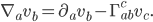
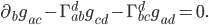
We want to find a way to use the metric to compare things at two different points.  In other words, the metric is a sort of standard measuring stick we want to use to see how other things change.  But obviously the metric cannot change relative to itself.  (If you define a yard as the length of a yardstick, then other things can change in size, but the stick will always be 1 yard by definition.)  Therefore, the covariant derivative of the metric itself is zero: $\nabla_c g_{ab} = 0$.  But if we write out the correction terms we get:

$$\nabla_c g_{ab} = \partial_c g_{ab} - \Gamma^{d}_{bc} g_{ad} - \Gamma^{d}_{ac} g_{bd} = 0.$$

We can use this equation to solve for $\Gamma$ in terms of the metric.  To do this, we just switch around the roles of the $a$, $b$, and $c$ indices to get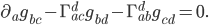

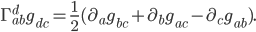
$$\partial_a g_{bc} - \Gamma^{d}_{ac} g_{bd} - \Gamma^{d}_{ab} g_{cd} = 0.$$

and

$$\partial_b g_{ac} - \Gamma^{d}_{ab} g_{cd} - \Gamma^{d}_{bc} g_{ad} = 0.$$

By adding up two of these equations and subtracting the other, and dividing by two, one can prove that

$$\Gamma^{d}_{ab} g_{dc} = \frac{1}{2}(\partial_a g_{bc} + \partial_b g_{ac} - \partial_c g_{ab}).$$

We can then define $\Gamma^{d}_{ab}$ directly as

$$\Gamma^{d}_{ab} = \frac{1}{2} g^{cd}(\partial_a g_{bc} + \partial_b g_{ac} - \partial_c g_{ab}).$$

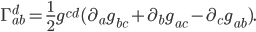
To do that, we had to introduce something called the inverse metric $g^{ab}$.  You get this by writing the metric $g_{ab}$ out as a matrix and inverting it.  (Technically we write $g_{ab} g^{bc} = \delta^c_a$ where $\delta^c_a$ is a very boring tensor which is always 1 if $a$ and $c$ are the same index, and 0 if they are different.)

So then, the connection (which allows us to transport vectors from place to place) can be written in terms of the first derivative of the metric.  We'll need to take a second derivative of the metric to get the curvature $R^{a}_{bcd}$, but that will be the subject of another post.