Curvature II: Spacetime

By Scott Church – Guest Blogger

In the first installment of this series, we explored the nature of curved spaces and introduced ourselves to some of the mathematical tools needed to describe how length, breadth, and height can be curved without higher dimensions to “curve into.” In the interest of keeping our exploration as intuitive as possible, we began with the Euclidean geometry we learned in high school and explored curvature from the vantage point of time as we experience it—a universal history that is the same for all of us and independent of the spatial stage on which our lives unfold. Today we will explore the nature of time and its relationship to space and discover (spoiler alert!) that in fact, it is neither separate from space nor absolute—not only can length, breadth, and height be curved, duration can be as well. The universe we inhabit is one of curved spacetime.

Special Relativity

The Newtonian physics we learned in high school presumes absolute three-dimensional space and time. In the low gravity and velocity world we live in, that is how we experience them. But intuitive as this may seem to us, there are hints that something is amiss. That physics also taught us that the speed of light $c$ is a universal constant that can be derived from Maxwell’s equations. And as we saw in Part I, the laws of physics, including $c$, must be invariant for all observers stationary or moving. Pause for a moment and reflect on what this implies. If I am standing beside a highway and you drive by at 50 mph, that is the speed I will observe. In the car, you will see yourself as stationary and the world passing you at 50 mph in the opposite direction, including me. Another driver doing 70 mph in the fast lane will pass me at that speed and you at 20 mph. But Maxwell’s equations will remain true and invariant for all observers, so if a beam of light is shined in the same direction, it will pass all three of us at the same speed. How is this possible?

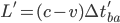
Imagine that you are now the one who is stationary, and I fly past you in a fighter jet at a speed $v$ of 3600 mph, (or one mile/sec for round numbers) carrying a clock that is in sync with an identical clock of yours. As I pass you, it emits a pulse of light in your direction at time $t_1$ which reaches your eye after travelling a distance $d_{t1}$ (Figure 1). One second later at $t_2$, a second pulse is emitted, but I will have flown one mile further so that pulse must travel a distance $d_{t2}$ before it reaches your eye. My clock will be ticking at the same rate in my reference frame as yours is for you, but the seconds you observe on my clock will be longer because the second pulse you receive from it must travel further at the same speed $c$ to reach your eye than the first one did. Your experience will be that my time runs slower for you than it does for me. And for the same reason, your clock will be running slower for me than it is for you.

Figure 1

As for distances, the length of my jet will be measured by the time it takes a pulse of light to travel from the nose ($A$) to the tail ($B$) at speed $c$ (Figure 2). In my reference frame that will be given by,

$L = c\Delta t_{ba}$                    [Eqn. 1]

 where $t_{ba}$ is my proper time (that is, the time measured by a clock at rest in my reference frame).

Figure 2

In your reference frame, the pulse of light will take a time $\Delta t^{'}_{ba}$ to travel the length of my jet. However, while the pulse is in transit, point $B$ will have moved forward a distance $v \Delta t{'}_{ba}$ so the pulse will arrive at point $B_2$ instead (Figure 3),

Figure 3

And you will observe the length of my jet to be the distance between $A$ and $B_2$, or,

$L^{'} = (c - v)\Delta t^{'}_{ba}$                    [Eqn. 2]

Not only will you see the pulse travelling a shorter distance that me, the time $\Delta t^{'}_{ba}$ will also be less than the $\Delta t_{ba}$ I observe because time is running slower for you than for me. The length $L^{'}$ you observe for my jet will be smaller than the length $L$ I observe, and you will see me and my jet as though we were compressed in the direction of travel.

Thus, we arrive at one of the foundational principles of special relativity; Space and time are neither absolute nor independent of each other. They’re united in a single spacetime manifold whose metric contains an underlying symmetry that preserves Maxwell’s equations and $c$ for all observers. And this manifold is not simply a map of locations and distances—it’s a frame-independent history of events for every location within it.

In Part I we saw that in the flat Newtonian universe of our experience, time is absolute and independent of space. All observers experience it the same, and spatial geometry is Euclidean with the interval between any two points is given by the Pythagorean Theorem,

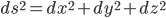 $ds^{2} = dx^{2} + dy^{2} + dz^{2}$                    [Eqn. 3]

In spacetime, however, this is no longer the case. Now we have a collection not of points, but events that reflect the histories of each spatial point within it. The interval no longer defines the distance from here to there; It defines here and now, to there and then. Accounting for this in our metric tensor won’t be as simple as it may sound. As we’ve seen, the speed of light must remain the same for all observers whether stationary or moving in any reference frame. And the relative motion slows time down and compresses space until both reach zero at the speed of light. From our vantage point, a photon’s reference frame is a single event with a zero-length interval, so our interval must include time with a sign opposite to that of space. After multiplying time by $c$ to convert it to equivalent distance units, this gives,

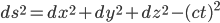$ds^{2} = dx^{2} + dy^{2} + dz^{2} - (ct)^{2}$                    [Eqn. 4]

Which adopting the usual (though not strictly necessary) convention of making time the first, or zero component, results in the spacetime metric tensor,

                              [Eqn. 5]

The diagonal terms expressed as a tuple, [-1, 1, 1, 1], is known as the metric’s signature. In differential geometry (the branch of mathematics that generalizes the geometry we learned in high school to all types of curves spaces), a continuous N-dimensional manifold that has a well-defined and positive-definite metric tensor at all points (not all mathematically possible ones do) is referred to as Riemannian. That is, a flat 4-D Riemannian metric is one that for every point on it, infinitesimal displacements in the locally flat tangent plane have a metric signature of [1, 1, 1, 1]. A universe with Euclidean geometry and absolute time would have this metric everywhere. But in a universe constrained by special-relativity the interval can be zero as well as positive, so the metric is non-degenerate rather than positive-definite. Manifolds of this type are referred to as pseudo-Riemannian.

In Part I, we conducted a geometric thought experiment in which we traversed a closed triangular path through the flat space of an observer named Freddy, and another through the curved space of an observer named Cathy along geodesics (paths that reflect the shortest distance between any two points). In each, we carried one vector with us while leaving an identical parallel copy of it behind and upon returning to point A. When we did this in Freddy’s flat space we found, not surprisingly, that after completing the journey the two vectors were still parallel to each other. But after the same journey through Cathy’s curved space, we discovered that the vector we carried with us was no longer parallel to the one we left behind even though both were still pointing in the same direction (globally south), and we had travelled a shorter distance that still encompassed a larger area. We introduced some mathematical concepts that allowed us to define a covariant derivative ¹ to describe the rate of change of the vector we carried with us along our path $s^{\sigma}$,

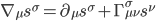$\nabla_{\mu}s^{\sigma} = \partial_{\mu}s^{\sigma} + \Gamma^{\sigma}_{\mu\nu}s^{\nu}$                    [Eqn. 6]

The first term on the right is the usual vector calculus gradient along the direction of travel. The second term, however, introduced a new object, the Christoffel symbol, that allowed us to map changes in the underlying tangent plane containing $s^{\sigma}$, itself onto local coordinate systems within it as we traversed the path. Integrating this derivative along our path would then fully capture the changes in our mobile vector with respect to its stationary twin we left behind.

That exercise, however, traversed a path through Cathy’s curved two-dimensional space, so equation 6 described distances and directions only. Had we included time in her curved universe, the path we walked would have been a trajectory of motion with history, and upon arriving back at A we would have found that our mobile vector was now older or younger than its stationary copy as well. In curved space, geodesics are the shortest distance between points—here and there. But in spacetime they are histories that reflect the shortest path, stationary or moving, between here and now, and there and then. As such, they define an equation of motion for the trajectory an object will follow when no forces are acting on it.

In a flat spacetime like Freddy’s, an object left to itself will remain stationary or move at constant velocity, so its geodesic will be a straight line whose slope will be the constant speed it is moving at. If one or more forces act on the object it will accelerate, and its history will follow a curved path whose velocity changes from moment to moment. We can derive the equation of motion for this by using equation 5 to derive the second order time derivative along $ds^{\sigma}$, to equate the acceleration produced by a force it to its strength divided by the object’s mass. In his flat spacetime, a single unvarying tangent plane spans the entire universe, so the Christoffel term will vanish, leaving us with,

$\frac{\partial^2 s^{\sigma}}{\partial t^2} = \frac{F}{m} = 0$                    [Eqn. 7]

Which we will recognize as a geodesic equation of motion for Newton’s second law that we learned in high school.

In Cathy’s universe things are different. There, geodesics are curved so the Christoffel term will generally be non-zero, and her equation of motion will be given by,

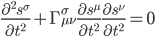$\frac{\partial^2 s^{\sigma}}{\partial t^2} + \Gamma^{\sigma}_{\mu\nu}\frac{\partial s^{\mu}}{\partial t^2}\frac{\partial s^{\nu}}{\partial t^2} = 0$                    [Eqn. 8]

Notice that in curved spacetimes like hers, the second term on the left will be non-zero even in the absence of forces, so the first term will be as well. Left to themselves, objects in a curved spacetime will experience freefall along accelerating trajectories.

Which brings us to the next topic…

General Relativity

The other hallmark of our high-school physics lessons was Newtonian gravity. In a universe of flat space and absolute time like Freddy’s, gravity is an attractive force between objects whose strength is a function of their masses and the distance separating them. Specifically, the gravitational force $F_g$ between two objects with masses $m_1$ and $m_2$ is given by,

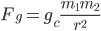$F_g = g_c\frac{m_1m_2}{r^2}$                    [Eqn. 9]

Where $r$ is the distance between their centers of mass and $g_c$ is the universal gravitational constant we also learned in our high-school physics classes.

For centuries this understanding of gravity has served us well in regions of low mass, velocity, and distance, and still does. I spent twenty years as an aerospace engineer designing commercial jet aircraft structures, and the aircraft my colleagues and I applied these principles to still have exemplary safety and performance records. But even so, physicists have long been troubled by the idea of “spooky action at a distance” forces. How can objects interact with each other invisibly over large distances? On the other hand, we can put it differently by saying that gravity causes objects with mass to accelerate toward each other at a rate given by their masses and the distance separating them, and as we saw above, freefall acceleration is a consequence of spacetime curvature. Jumping the gun, we also know that mass and energy are equivalent (hence Einstein’s celebrated $E = mc^2$) and moving objects with mass have a kinetic energy that is a function of their momentum and mass ($K = p^2/2m$). This raises an interesting question…

What if gravity isn’t a force at all, but simply a local manifestation of spacetime curvature due to mass, energy, and momentum?

If this is true, then we would expect that two objects of differing mass in the field of a third object of much larger mass (like the earth, for instance) would experience the same freefall acceleration toward it—essentially, that the “force” $F_g$ the gravitational field exerts on their differing small masses would result in the same acceleration for both,

$\frac{F_{g1}}{m_1} = \frac{F_{g2}}{m_2}$                    [Eqn. 10]

And this would be the same acceleration that would result from an equal but non-gravitational force (e.g. - the thrust produced by a rocket engine). As you’ve probably guessed by now, this is the case. Gravitational mass and inertial mass are indistinguishable from each other, and freefall accelerations induced by the former are a consequence not of any “spooky action at a distance” force, but of the local spacetime curvature created by its presence. This identity, known as the equivalence principle, is the heart and soul of general relativity. Throw a pebble into a pond and watch it arc through the summer sky before splashing down, and you are literally seeing the curvature of length, height, breadth, and duration where you’re standing because of the mass of the earth beneath your feet! ²

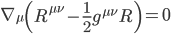
And once again, if spacetime curvature is caused by mass, energy, and momentum, we can ask ourselves how this could be captured mathematically. As in Part I, a formal derivation of the relationship between the two is beyond the scope of an introduction to the topic, but we can introduce the types of mathematical objects needed and how they relate to each other. The first thing we need is an object that describes curvature. Like the terms introduced so far, it will need to capture the change in angles over infinitesimal displacements from any reference frame we view it from, so it will need to be a covariant or contravariant tensor. And since we want it to describe curvature specifically rather than displacements, it will be a function of the Christoffel symbols that describe how they change when we walk a parallel transport path (or more properly, a function of their first derivatives, or rates of change). To unambiguously capture this, we will have to carry a four-vector $ds$ (that is, a vector in three spatial dimensions plus time) around an enclosed path for which all the interior angles are orthogonal to each other (locally 90 degrees). Previously, we were able to do this with a triangular path in Cathy’s space because for clarity of the underlying principles we presumed it to be spherically curved, but that won’t be true of curved spacetime in general. So, now we must carry our four-vector along a four-legged parallel transport path (presumed to be infinitesimally small for a local curvature description), again preserving its local orientation at every point, as shown in Figure 4 (Wikimedia, 2015).

Figure 4

Upon returning to our starting point, we will have a function that describes how each of the four components of $ds$ changed with respect to the others for each of the four legs of the journey. As such it will be a tensor with four indices (rank 4) each of which covers four dimensions, so it will have $4^4$, or 256 components. This tensor, known as the Riemannian curvature tensor $R^{\mu}_{\nu\rho\sigma}$, fully describes the actual curvature of spacetime at every point on the manifold. It can be specified in covariant or contravariant terms, but since it captures how a contravariant vector is affected by local covariant curvature, it’s customary to express it with one “upstairs” index and three “downstairs” ones, as shown here.

Before going any further, there are two related tensors we’re going to need (why will become apparent shortly). In Part I we discussed how a tensor object defined by N indices can be “contracted” to fewer indices by projecting one or more of the index’s components onto the others—in essence, “averaging” it into the remaining ones. For a tensor expressed in covariant form for all indices, we do this by multiplying it by the contravariant metric tensor in one or more of its indices. Contracting the Riemann tensor in this manner for two of its four indices gives,

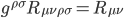 $g^{\rho\sigma}R_{\mu\nu\rho\sigma} = R_{\mu\nu}$                    [Eqn. 11]

The resulting tensor, $R_{\mu\nu}$, is known as the Ricci tensor. Contracting it again on both of its indices yields the Ricci scalar, $R$. These have different physical interpretations. The Ricci tensor describes the rate of change of an infinitesimal element of spacetime volume along $ds$ due to tidal forces. That is, as we move through spacetime along a group of infinitesimally separated parallel geodesics, it describes how an element of volume between them changes in each direction. The Ricci scalar, on the other hand, gives a non-dimensional measure of how the overall enclosed volume itself changes.

Next, we need a tensor object that describes the mass, energy, and momentum we suspect to be curvature’s source. That tensor (which we won’t make any attempt to formally derive here), is known as the stress energy momentum tensor, $T^{\mu\nu}$. Its components are defined in a manner similar to those of the metric tensor, $g_{\mu\nu}$, but using momentum density four-vectors (momentum density in three spatial dimensions plus energy density, which can be thought of as “momentum” in time for a stationary object). Because its momentum density components are vectors, it is customary to express it in contravariant form (indices “upstairs”). The first index ($\mu$) gives the four-momentum components being considered, and the second ($\nu$) gives the direction it is being compared to. The physical significance of its components is as shown in Figure 2 (Wikimedia, 2013).

Figure 5 – The Stress Energy Momentum Tensor

With these tools in hand, we can proceed with our investigation of how mass, energy, and momentum curve space and time, but there are still a few constraints we need to account for.

First, the stress energy momentum tensor is rank 2 but the Riemann curvature tensor is rank 4 (that is, the former has two indices with 16 components, whereas the latter has 4 indices and 256 components), so we can’t just equate them to each other. Whatever effect $T^{\mu\nu}$ has on curvature will have to manifest itself as a rank 2 curvature object as well—that is, it will have to be a contraction of the Riemann tensor that reflects the behavior we observe in gravity, so we want to know what sort of contraction will give us that.

We saw earlier that in the absence of forces, spacetime curvature manifests as acceleration. Strictly speaking, this applies only to point masses in the gravitational field of a much larger mass. For objects that have size and shape, the story changes. In Newtonian physics, the gravitational force between two masses varies inversely as the square of the distance between them (equation 9). So, if you are falling toward the earth feet first, your feet are being pulled harder than your head because they are closer to the earth’s center of gravity. Inasmuch as this is the low mass/energy/momentum limit of GR, the same will be true in curved spacetime as well. Likewise, your freefall into the earth’s gravitational well will be along a geodesic, and the deeper you go, the closer adjacent geodesics to your sides will be. Figure 3 (Wikimedia, 2008) shows what a gravitational well created by a mass as the bottom of the “pocket” looks like.³ The longitudinal lines are freefall geodesics with their steepness at each node being the strength of gravity there, and the squares enclosed by the grid can be thought of as shapes.

Figure 6 – Gravitational Well

Notice how falling into the well squeezes the latitudinal rectangles into increasingly longitudinal ones. In the earth’s relatively weak gravitational field compared to your size, the effect is too small to notice. But as you fall toward it, feet-first, you are being stretched and squeezed. This stretching and squeezing of large objects are tidal forces, and in the limit of a point mass, they reduce to simple freefall acceleration. Since in the most general terms, tidal forces are how curvature manifests, we would expect the stress energy momentum tensor to equate to a rank 2 tensor that describes them. And as we’ve seen, we have one… the Ricci tensor!

But we’re not out of the woods yet. There is one more constraint we need to honor; Another of the fundamental ones we learned in our high school physics, conservation of energy and momentum. Although neither is well-defined nor self-evidently conserved for the whole universe (or large regions of it), for locally flat inertial reference frames in the tangent planes of every point in it, both need to be conserved. This means that for every point on the manifold the divergence of the stress energy momentum tensor must be zero. That is,

$\nabla_{\mu}T^{\mu\nu} = 0$                   [Eqn. 12]

And here we have a problem… Tidal forces do not vanish in locally flat regions, and neither does the divergence of the Ricci tensor. If they did, falling through a black hole event horizon would be a lot less traumatic! So, our contracted curvature tensor object is going to need some tweaking.

Fortunately, the full Riemann curvature tensor itself gives us a way out. As it happens, its own internal consistency does require it to vanish locally; When curvature vanishes (as it must in local tangent planes) so does the curvature tensor. One consequence of this is that the sum of its divergences with respect to any three of its four indices must add to zero. That is,

$\nabla_{\mu}R^{\mu }_{ \nu\rho\sigma} + \nabla_{\nu}R^{\nu}_{\mu\rho\sigma} + \nabla_{\rho }R^{\rho}_{\mu\nu \sigma} = 0$                   [Eqn. 13]

This relationship is known as the second Bianchi identity (of which there are several). Again, we needn’t worry about its formal derivation here. But for our purposes, what matters is that with some mathematical gymnastics we can derive from it the contracted Bianchi identity,

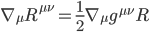$\nabla_{\mu}R^{\mu\nu} = \frac{1}{2}\nabla_{\mu}g^{\mu\nu}R$                   [Eqn. 14]

 Gathering terms gives,

$\nabla_{\mu}\left ( R^{\mu\nu} - \frac{1}{2}g^{\mu\nu}R \right ) = 0$                   [Eqn. 15]

And finally, by combining the Ricci tensor for tidal forces and the Ricci scalar for volumetric curvature, we have a tensor object we can equate to the stress energy momentum tensor that captures the spacetime curvature it induces while sharing with it a zero divergence that locally preserves conservation of energy and momentum. It’s customary to refer to the term in brackets as the Einstein tensor $G^{\mu\nu}$, from which we have,

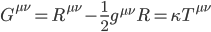$G^{\mu\nu} = R^{\mu\nu} - \frac{1}{2}g^{\mu\nu}R = \kappa T^{\mu\nu}$                   [Eqn. 16]

Where $\kappa$ is a proportionality constant which again, we won’t derive here, but turns out to be,

$\kappa = \frac{8\pi g_c}{c^4}$                   [Eqn. 17]

And there you have it, Ladies and Gentlemen… an equation that relates mass, energy, and momentum to spacetime curvature, and therefore gravitation!

One final question remains. Technically, equation 16 is arbitrary to within an additive constant as well. When Einstein first derived this relationship, he realized that it predicted a universe that was necessarily expanding or contracting, and thus impermanent. The idea of a universe that wasn’t eternal was philosophically abhorrent to him, so he included a constant term on the left (typically denoted with the Greek letter $\Lambda$), multiplied by the metric tensor for consistency and sized to offset the expansion, thereby preserving a curved, but static and eternal universe. Later, when it was independently confirmed that the universe is in fact, expanding (a fascinating story in its own right!), Einstein retracted the constant calling it “the greatest mistake of my life.” But as it turns out, it wasn’t. It has since been discovered that the cosmological constant is not only real, but positive and causing the expansion of the universe to accelerate! The discovery was so striking that the leaders of the team who discovered it, Saul Perlmutter, Brian Paul Schmidt, and Adam Guy Riess were jointly awarded the 2011 Nobel Prize in physics.

So… combining equations 16 and 17 with all terms expressed as covariant (which is customary), and restoring the cosmological constant to its rightful place we have,

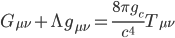$G_{\mu\nu} + \Lambda g_{\mu\nu} = \frac{8\pi g_c}{c^4} T_{\mu\nu}$                   [Eqn. 18]

These are the celebrated Einstein Field equations that are the hallmark of general relativity. The terms on the left fully describe the geometry of spacetime for all observers at every point in the universe, and the term on the right describes the mass, energy, and momentum that produces that geometry.

This was meant to be an introduction to spacetime curvature, so we’ve arrived at them with some big leaps and little in the way of formality. Though at first blush they may seem daunting and difficult to wrap your mind around, the important thing for today is an understanding of what the terms in these equations mean, and why they must have the general forms they do to describe how length, height, breadth, and duration can be curved. For those who want to explore further, there any number of good introductions to general relativity for the layperson. One that I found particularly readable and informative was Clifford Will’s book Was Einstein Right – Putting General Relativity to the Test (1993), first published in 1986 when I was in grad school. If you feel ready to make the deep dive into the full formalism of general relativity, there are many textbooks on the subject. But if there is one that has stood for many years as the Bible of general relativity, it’s Misner, Thorne, and Wheeler's Gravitation (2017). It’s rigorous and will take some time to wade through, but it’s the best, and most thorough general relativity course I am personally aware of and has been since it was first published in 1973.

The psalmist tells us,

“The heavens are telling the glory of God; and the firmament[a] proclaims his handiwork. Day to day pours forth speech, and night to night declares knowledge. There is no speech, nor are there words; their voice is not heard; yet their voice goes out through all the earth, and their words to the end of the world.” – Psalm 19:1-4

When I gaze up at the nighttime sky, I see stars that are hundreds of light years away, many of which are surrounded by worlds, possibly even worlds not unlike my home. And I realize that I’m gazing upon those stars and worlds not as they are now in my reference frame, but as they were centuries ago. If I were to turn a large enough telescope on that sky I would see galaxies, quasars, nebulae, and a bewildering spectacle of other wonders, some of which are billions of years old and revealing themselves to me from a time long before humans or even our solar system existed. And if I filter their light through a spectrometer, I will see the fingerprints of their chemical constituents shifted increasingly toward the red the more distant they were, and I would realize that I was watching the universe grow—not as an expansion of matter into a pre-existing void, but literally the expansion of space and time themselves from a cataclysmic birth 13.73 billion years ago. I would see in that the glory of God and his handiwork…

And I would suspect, as J.B.S. Haldane did a century ago, the handiwork of God, where length, breadth, height, and duration are themselves clay in His artistic hands, is not only queerer than I suppose, but queerer than I can suppose.

Footnotes

1)  In Part I we introduced the nabla symbol on the left ($\nabla_{\mu}$), which in mathematics is known as the Laplace operator. It is a shorthand reference for the gradient (first derivative) in the direction of a vector defining the $\mu$ coordinate system. That is, 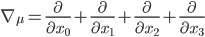$\nabla_{\mu} = \frac{\partial }{\partial x_0} + \frac{\partial }{\partial x_1} + \frac{\partial }{\partial x_2} + \frac{\partial }{\partial x_3}$ where the index $\mu$ = 0, 1, 2, 3. This representation of a gradient in a particular direction is also referred to as the divergence.

2)  Interestingly, this isn’t just theoretical. Google and Apple map apps leverage first-order corrections for spacetime curvature near the earth’s surface to refine the accuracy of your location from raw GPS triangulated signals. General relativity is literally why your phone knows your location to within a couple hundred feet or so rather than one or two city blocks!

3)  Strictly speaking, this is a 2-D gravitational well with absolute time rather than a true 4-D gravitational which would include time. But for the current purpose, it suffices to illustrate the point.

References

Misner, C.W., Thorne, K.S. & J.A. Wheeler. 2017. Gravitation. Princeton University Press (Oct. 24, 2017). ISBN-10: 9780691177793, ISBN-13: ‎978-0691177793. Online at https://www.amazon.com/Gravitation-Charles-W-Misner/dp/0691177791/ref=sr_1_1?crid=1OKXLNQA5YVAR&keywords=gravitation&qid=1694219167&sprefix=gravitation%2Caps%2C253&sr=8-1&ufe=app_do%3Aamzn1.fos.18630bbb-fcbb-42f8-9767-857e17e03685.  Accessed Oct. 9, 2023.

Wikimedia. 2008. Image courtesy of AllenMcC. Based on the work of Bamse, and Melchoir, CC BY-SA 4.0, Mar. 2, 2013. Online at https://commons.wikimedia.org/wiki/File:GravityPotential.jpg. Accessed Oct. 9, 2023.

Wikimedia. 2013. Image courtesy of Maschen. Based on the work of Bamse, and Melchoir, CC BY-SA 4.0, Mar. 2, 2013. Online at https://commons.wikimedia.org/w/index.php?curid=24940142. Accessed Oct. 9, 2023.

Wikimedia. 2015. Image courtesy of IkamusumeFan, CC BY-SA 4.0, Jan. 1, 2015. Online at https://commons.wikimedia.org/w/index.php?curid=2615879. Accessed Oct. 9, 2023.

Will, C.N. 1993. Was Einstein Right? - Putting General Relativity to the Test. Basic Books; 2nd edition (June 2, 1993). ISBN-10: ‎0465090869; ISBN-13: ‎978-0465090860. Online at https://www.amazon.com/Was-Einstein-Right-Putting-Relativity/dp/0465090869/ref=sr_1_1?crid=TOG1ZAWGPF20&keywords=was+einstein+right&qid=1696883510&sprefix=was+einstein+right%2Caps%2C171&sr=8-1. Accessed Oct. 9, 2023.